4.3 Position vs. time graphs
Let’s look at an object whose motion along a single dimension (for example, only moving forward/backwards) is described by the graph on the left in the figure below.

Position vs. time graph 
Velocity vs time graph
What does this graph tell us? It tells us where the object is at any given moment in time. For example, we know that at a time of 0.5 s, the object had a position of 5 m. Conversely, we could ask “at what time does the object have a position of 30 m?” Looking at the graph tells us that the object has a position of 30 meters at a time of 3 seconds.
Finally, we can see that our definition of velocity (change in position divided by change in time) is the slope of the position vs. time graph. In this case, it looks like the velocity of the object is (choosing the two points that we just looked at):
\[
v = \frac{30 – 5}{3 – 0.5}\frac{\textrm{m}}{\textrm{s}} = 10\ \textrm{m/s}
\]
Determining velocity from a position vs time graph
So, we can look at a graph of position vs. time, and analyze the velocity. From this information, we can plot a graph of velocity vs. time. For example, in the graph we were just looking at, the slope of the line is not changing; the slope is constant. This means the object was moving at a constant velocity. So a velocity vs. time graph would be a horizontal line, indicating the velocity is the same for all points in time. This would look like the graph on the right in the figure above.
An object may move in a series of constant-velocity movements. An example of such motion could be when you get up from your desk and start walking in one direction, then forget why you got up and turn around to go back to your desk, then suddenly remember again and turn back around to walk in the direction you were originally going. When this is the case, you can determine the velocity of the object for each interval of time, and your velocity vs time graph would be a series of horizontal lines.
Example 4.3
The graph below shows a position vs time graph representing the motion of an object moving in one dimension. There are several intervals of time over which the velocity is constant; for each interval determine the velocity. Plot a graph of velocity vs time.
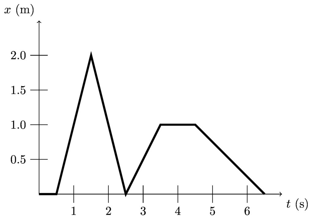
Velocity is the rate of change of position, the slope of a position vs. time graph. The slope of each straight line can be determined by “rise over run.” In this case, the “rise” is the change in position and the “run” is the change in time.
From time 0 seconds to 0.5 seconds, the velocity is
\[
\begin{align}
v_1 &= \frac{\Delta x_1}{\Delta t_1} \\
&= \frac{0 – 0}{0.5} \\
&= 0
\end{align}
\]
From time 0.5 s to 1.5 s, the velocity is
\[
\begin{align}
v_2 &= \frac{\Delta x_2}{\Delta t_2} \\
&= \frac{2 – 0}{1} \\
&= 2\ \textrm{m/s}
\end{align}
\]
From time 1.5 s to 2.5 s, the velocity is
\[
\begin{align}
v_3 &= \frac{\Delta x_3}{\Delta t_3} \\
&= \frac{0 – 2}{1} \\
&= -2\ \textrm{m/s}
\end{align}
\]
And so on. From time 2.5 s to 3.5 s the velocity is 1 m/s; from time 3.5 to 4.5 s the velocity is 0; and from time 4.5 s to 6.5 s the velocity is -0.5 m/s. For each interval of time, the velocity is constant. The velocity vs time graph looks like
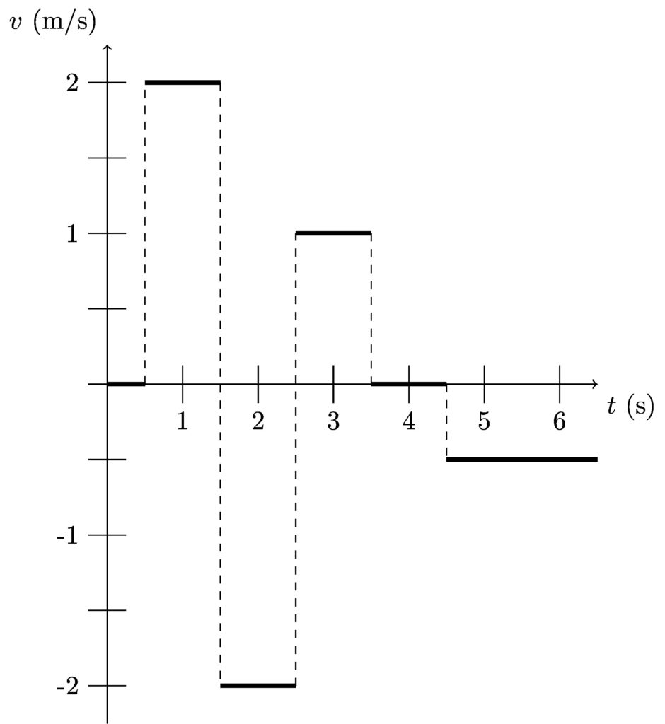
Both the position vs time and velocity vs time graph indicate that the object changed velocity instantaneously. The position vs time graph shows this by the abrupt change in slope of the line, and the velocity vs time graph shows this by the lines jumping from one velocity to another. In reality, velocity does not change instantaneously; there is some transition as the object changes from moving at one velocity to another. A jagged position graph like the one we started with would be the result of not recording a sufficient amount of data.
More realistic graphs would be smoothed out, as shown below.

Position vs time 
Velocity vs time