In the previous section we applied a test to see if a variable was bound in the body of a function. We haven’t seen many examples so far where this would be true, but consider function (λx. + (λy. + 3 y) x 2); is y bound in it?
We consider the function to be: (λx. E) so clearly, y doesn’t appear in the parameter list. The other possibility is that it is bound in E. Here, E = (+ (λy. + 3 y) x 2). This time y does appear in the parameter list, and it is free in the body (+ 3 y), meaning that it is bound in E, so it follows that y is bound in (λx. + (λy. + 3 y) x 2).
This is a fairly subtle thing, so make sure you’re satisfied with this before going on. What this tells us is that a variable doesn’t have to be bound by the first λ in an expression, that it can be bound elsewhere in the expression.
If we try evaluate that function by passing it the value 7 we get:
( (λx. + (λy. + 3 y) x 2) 7)
Perform a \(\beta\) conversion on x to get:
(+ (λy. + 3 y) 7 2)
Now we do another \(\beta\) conversion (on y) to get:
(+ (+ 3 7) 2)
Here’s another example. Is x free or bound?
((λx. + x 3) x)
If we take E to be (λx. + x 3) and F to be x, then x is bound in E and free in F, which means that x is both free and bound in (E F), so it is free and bound in the same expression! What does this mean? It means that these are two different x‘s, so the same name doesn’t always mean the same variable. Take a look at the AST below; it’s much clearer there because the λ node shows us which x belongs to the parameter list.
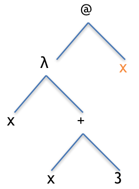
An AST with two different variables that have the same name.
Here’s another more complex example:
((λf. f (* 1 3) (+ 4 5) x) ((λxyz. (* 2 x)))
Which x is free and which bound? If we apply our rules then we can see that is is both. It is free in the (λf. f (* 1 3) (+ 4 5) x) part, and bound in the (λxyz. (* 2 x)) part.
Here it is as an AST:
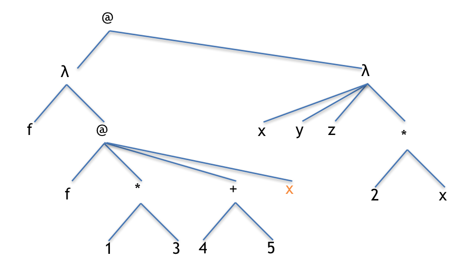
A function calling another function. The orange x is a free variable that will need a value.
The first thing we do is to bring in the value for f as below:
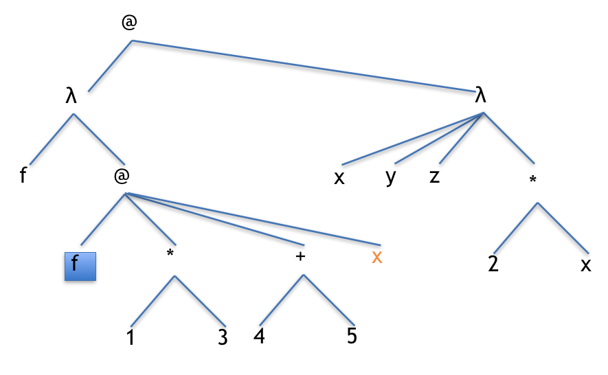
The variable to be replaced.
This \(\beta\) reduction gives us this:
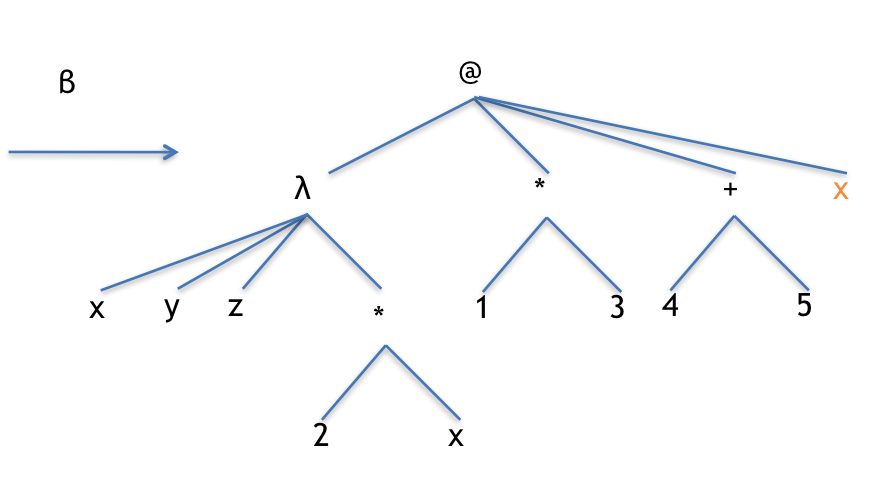
The AST after applying the beta reduction.
Now we’re stuck. We have a λ expression that takes three parameters and, although we have three, the orange x is free, so let’s assume it has been define somewhere else like this:
(define x 2)
That changes the AST to this, which has enough arguments so we can apply our \(\beta\) reduction.
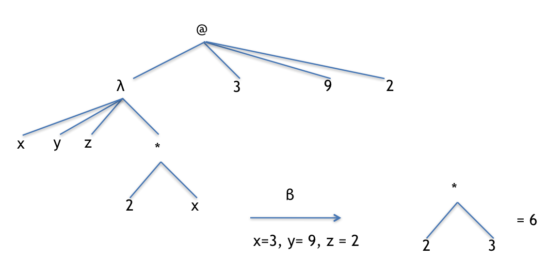
The final steps of the reduction.
Recall from the section on Lifetime Diagrams that internally, the computer uses different names for variables:

A Lifetime Diagram with multiple copies of the same function running.
This shows how the names can be easily kept separate when there are multiple copies of the same function running. This is important because in that case, there will definitely be functions using the same name, but what if we pass a function to another function like we did above? It turns out that it’s the same thing; any time a function is actually running, a temporary variable is set up to keep that function’s values private to it. However, when we’re reading these functions written out in λ calculus, it won’t always be that clear, so let’s add some more formal notation to help us keep everything straight.
We’ve been using \(\beta\) reductions for a while now. Formally, a \(\beta\) reduction replaces the free occurrences of a variable in the body of a function. For example, in the expresion ((λx. + x 1) 5) we will replace all the free occurrences in the body (+ x 1) with the value 5, giving us (+ 5 1). Formally, we write this as:
\( ((\lambda x. + x\; 1)\; 5) \overrightarrow\beta (+ 5\; 1)\)Here’s a more complex example, this time with multiple λ expressions:
\( ((\lambda x. + (\lambda y. +\; 2\; y)\; x\; 4)\; 3)\)Our \(\beta\) reduction does the following:
\( \overrightarrow\beta (+ (\lambda y. +\; 2\; y)\; 3\; 4)\)Next we do another one to get:
\( \overrightarrow\beta (+\; (+\; 2\; 3)\; 4)\)Note that we haven’t added anything new here, we’ve just formalised what we’ve been doing for a while now, which is bringing in values for parameters. Here’s a more confusing but identical example:
\( ((\lambda x. + (\lambda x. +\; 2\; x)\; x\; 4)\; 3)\)When we do our \(\beta\) reduction we only replace the free occurrences of x, and the inner λ has a bound x, so that doesn’t change, giving us:
\( \overrightarrow\beta (+ (\lambda x. +\; 2\; x)\; 3\; 4)\)Yes, it still looks slightly different to the last example, but only the names are different. Structurally and functionally it is the same, that is, semantically it is the same even though the syntax is different.
We’ll finish up with one last mind-bending example of passing a λ expression to another λ expression. This might seems a strange thing to want to do, as so far we’ve only modified the functionality of something by passing it a different piece of data; however, what this will let us do is modify the functionality of a piece of code by passing it another piece of code! Think about the parallel processing examples we had before, this is a really great way to change the functionality of a system very quickly.
Let’s start with (λf. f 3) (λx. + x 1).
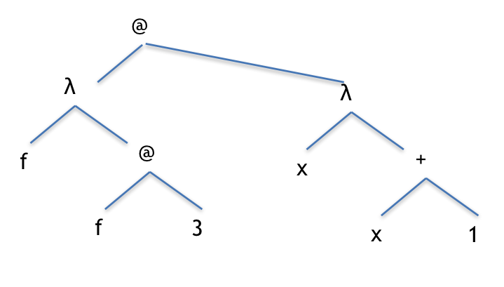
Passing a lambda expression into another lambda expression.
Next we do our \(\beta\) conversion
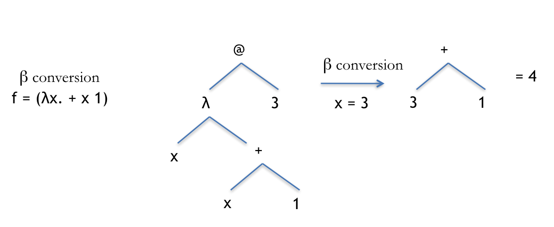
Perform a beta conversion (reduction) on the AST, followed by another one on the remaining tree.
Well, that was actually disappointingly easy and straightforward, so let’s try a different one!
(λx. + 2 (λy. y 5) x) (λz. + 1 z)
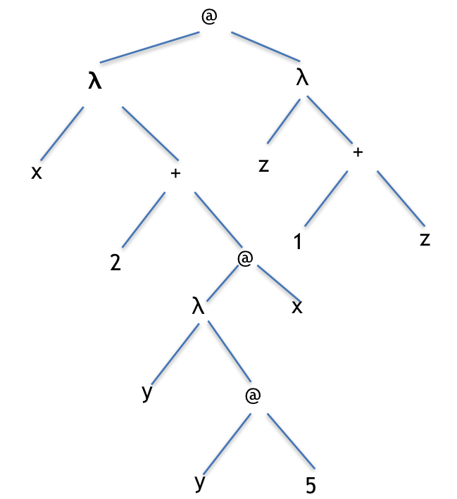
An expression with three lambda expressions!
We apply the first one and perform a \(\beta\) conversion
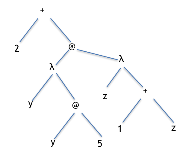
Perform a beta reduction. Notice that the + is now on top.
Now we bring in the subtree for y
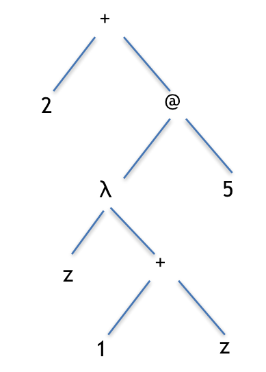
Perform another beta reduction to leave us with just one lambda expression. Notice that the + is still on top.
Now we do our final one to get a good old fashioned AST that is ready to be reduced to a single value.
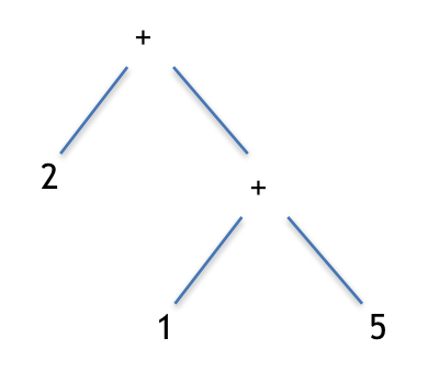
The final AST, ready for reduction to a single number.
Now, that was way more interesting!